Consumption Linear Regression Example

Requirements

Get the required libraries.

library(AER)

## Loading required package: car
## Loading required package: lmtest
## Loading required package: zoo
## 
## Attaching package: 'zoo'
## 
## The following objects are masked from 'package:base':
## 
##     as.Date, as.Date.numeric
## 
## Loading required package: sandwich
## Loading required package: survival
## Loading required package: splines

library(MASS)
library(car)
data("USMacroG")

Data Exploration

Get the differences per column

MacroDiff = apply(USMacroG, 2, diff)

Plot data that we are interested in

subset <- cbind(MacroDiff[,"consumption"], 
                MacroDiff[,"dpi"], 
                MacroDiff[,"cpi"], 
                MacroDiff[,"government"], 
                MacroDiff[,"unemp"])
colnames(subset) <- c("consumption", "dpi", "cpi", "government", "unemp")
df <- as.data.frame(subset)
pairs(df)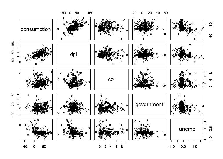

Linear Regression Analysis

We want to predict consumption based on the other variables. Some of the more correlated variables are dpi (real disposable personal income) and unemployment

Fit a linear model using the other four varables

fit.lm1 = lm(df$consumption~df$dpi+df$cpi+df$government+df$unemp)
summary(fit.lm1)

## 
## Call:
## lm(formula = df$consumption ~ df$dpi + df$cpi + df$government + 
##     df$unemp)
## 
## Residuals:
##     Min      1Q  Median      3Q     Max 
## -60.626 -12.203  -2.678   9.862  59.283 
## 
## Coefficients:
##                 Estimate Std. Error t value Pr(>|t|)    
## (Intercept)    14.752317   2.520168   5.854 1.97e-08 ***
## df$dpi          0.353044   0.047982   7.358 4.87e-12 ***
## df$cpi          0.726576   0.678754   1.070    0.286    
## df$government  -0.002158   0.118142  -0.018    0.985    
## df$unemp      -16.304368   3.855214  -4.229 3.58e-05 ***
## ---
## Signif. codes:  0 '***' 0.001 '**' 0.01 '*' 0.05 '.' 0.1 ' ' 1
## 
## Residual standard error: 20.39 on 198 degrees of freedom
## Multiple R-squared:  0.3385, Adjusted R-squared:  0.3252 
## F-statistic: 25.33 on 4 and 198 DF,  p-value: < 2.2e-16

confint(fit.lm1)

##                     2.5 %     97.5 %
## (Intercept)     9.7825024 19.7221311
## df$dpi          0.2584219  0.4476652
## df$cpi         -0.6119382  2.0650912
## df$government  -0.2351363  0.2308197
## df$unemp      -23.9069164 -8.7018187

Looking at the Pr(>|t|) values within the summary of the fitted linear model, dpi and unemp are much smaller than the other two varables, and dpi and unemp are small, giving evidence that the corresponding coefficient is not 0 and that they have a linear relationship with consumption.

The p values for cpi and government are large, so we would not reject the null hypothesis that the coefficients for cpi and government is 0.

In other words, we can accept the null hypothesis that consumption and cpi are not linearly related and that consumption and government are not linearly related, given that we have dpi and unemp. Note that without dpi and unemp, consumption and either cpi or government might be highly correlated and linear in a regression analysis.

Print an Analysis of Variance Table

anova(fit.lm1)

## Analysis of Variance Table
## 
## Response: df$consumption
##                Df Sum Sq Mean Sq F value    Pr(>F)    
## df$dpi          1  34258   34258 82.4294 < 2.2e-16 ***
## df$cpi          1    253     253  0.6089    0.4361    
## df$government   1    171     171  0.4110    0.5222    
## df$unemp        1   7434    7434 17.8859 3.582e-05 ***
## Residuals     198  82290     416                      
## ---
## Signif. codes:  0 '***' 0.001 '**' 0.01 '*' 0.05 '.' 0.1 ' ' 1

The Sum Sq is interesting in that it measures the proportion of variance in consumption that can be linearly predicted by the variables.

Order matters in this analysis. We tend to want to put the most relevant toward the top, because without the other predictors for example, cpi may have more of a correlation than it does when the other variables are considered.

This calls for some intuative assumptions. For this analysis, I assume that dpi and unemp are more personal, or directly related to the individual, and would have more effect on consumption, so they should be at the top.

Reorder data for the linear regression model

fit.lm1 <- lm(df$consumption~df$dpi+df$unemp+df$cpi+df$government)
anova(fit.lm1)

## Analysis of Variance Table
## 
## Response: df$consumption
##                Df Sum Sq Mean Sq F value    Pr(>F)    
## df$dpi          1  34258   34258 82.4294 < 2.2e-16 ***
## df$unemp        1   7381    7381 17.7590 3.808e-05 ***
## df$cpi          1    476     476  1.1465    0.2856    
## df$government   1      0       0  0.0003    0.9854    
## Residuals     198  82290     416                      
## ---
## Signif. codes:  0 '***' 0.001 '**' 0.01 '*' 0.05 '.' 0.1 ' ' 1

Since significance of the others change when a variable is removed, we will remove one at a time.

fit.lm2 <- stepAIC(fit.lm1)

## Start:  AIC=1228.98
## df$consumption ~ df$dpi + df$unemp + df$cpi + df$government
## 
##                 Df Sum of Sq    RSS    AIC
## - df$government  1       0.1  82291 1227.0
## - df$cpi         1     476.2  82767 1228.2
## <none>                        82290 1229.0
## - df$unemp       1    7433.5  89724 1244.5
## - df$dpi         1   22499.9 104790 1276.0
## 
## Step:  AIC=1226.98
## df$consumption ~ df$dpi + df$unemp + df$cpi
## 
##            Df Sum of Sq    RSS    AIC
## - df$cpi    1     476.5  82767 1226.2
## <none>                   82291 1227.0
## - df$unemp  1    7604.2  89895 1242.9
## - df$dpi    1   22542.0 104833 1274.1
## 
## Step:  AIC=1226.15
## df$consumption ~ df$dpi + df$unemp
## 
##            Df Sum of Sq    RSS    AIC
## <none>                   82767 1226.2
## - df$unemp  1    7380.8  90148 1241.5
## - df$dpi    1   22931.9 105699 1273.8

summary(fit.lm2)

## 
## Call:
## lm(formula = df$consumption ~ df$dpi + df$unemp)
## 
## Residuals:
##     Min      1Q  Median      3Q     Max 
## -60.892 -12.660  -3.065   9.737  59.374 
## 
## Coefficients:
##              Estimate Std. Error t value Pr(>|t|)    
## (Intercept)  16.28476    1.91084   8.522 3.79e-15 ***
## df$dpi        0.35567    0.04778   7.444 2.84e-12 ***
## df$unemp    -16.01489    3.79216  -4.223 3.66e-05 ***
## ---
## Signif. codes:  0 '***' 0.001 '**' 0.01 '*' 0.05 '.' 0.1 ' ' 1
## 
## Residual standard error: 20.34 on 200 degrees of freedom
## Multiple R-squared:  0.3347, Adjusted R-squared:  0.3281 
## F-statistic: 50.31 on 2 and 200 DF,  p-value: < 2.2e-16

We were right to want to remove cpi and government.

Let’s plot the partial residual plots to see the relationship between the least-squares line (dashed red line) and the lowess curve (solid green line)

par(mfrow=c(2,2))
sp <- 0.8
crPlot(fit.lm1, df$dpi, span=sp, col="black")
crPlot(fit.lm1, df$cpi, span=sp, col="black")
crPlot(fit.lm1, df$government, span=sp, col="black")
crPlot(fit.lm1, df$unemp, span=sp, col="black")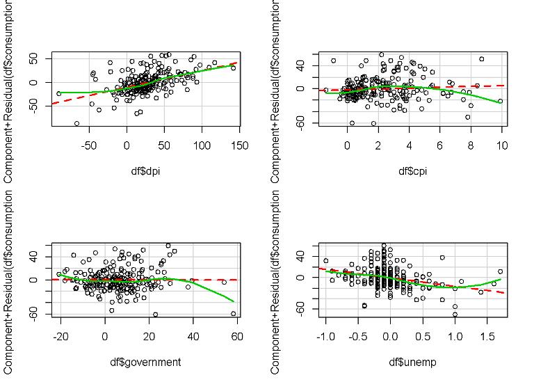

The deviation of the least-squares and lowess curve of the cpi suggest that the predictor is not linear.