Insights into data
Facebook Stock Price after Quarterly Report
Last week, Wednesday after the close, Facebook reported a stellar quarter, beating analysts’ expectations by at least 10%, yet the stock price is falling after the initial surge. Is this the normal behavior for this stock?
We will take a closer look by reviewing the plans and strategies described in the latest conference call and performing some basic stats on the price after the report.
Summary of the conference call
Mark Zuckerberg repeatedly mentioned video first. The phrase likely stems from the development strategy mobile first, where developers and designers focus on the mobile experience first (partly because of the rise in use of mobile devices, but mostly because of connectivity issues and resource limitations). The theory is that if you get the app to work for mobile, then the app will work on other devices.
So what is video first? Mark mentioned that he likes to think of the platform, or the app or the feature as stages. For example, the first stage is to focus on the user experience. So in this stage, they are likely focused on connectivity, allowing the video to play after a connection loss, and serving the highest quality based on connection speed and device (likely many more issues that I am not aware of). Also in this first stage, Facebook seems to add new features that the user will use and more easily create video content, such as Facebook Live. Another new feature I expect to see soon is a video chat. Facebook is focused on connecting users, so video chat makes sense. The second stage would likely be connecting the users to businesses in a seemingly natural way, and the third stage allowing businesses to monetize with video.
Facebook’s strategy makes sense, and it worked for mobile, so it will likely work for video and VR. That part of the conference call doesn’t signal any red flags.
Facebook Report Dates
It looks like FB reported on the following dates after the close:
- Jul 27, 2016 (28th was the first day of trading)
- Apr 27, 2016 (reported date)
- Jan 27, 2016 (reported date)
- Nov 4, 2015 (reported date)
- Jul 29, 2015 (reported date)
- Apr 22, 2015 (reported date)
- Jan 28, 2015 (reported date)
- Oct 28, 2014 (reported date)
- Jul 23, 2014 (reported date)
- Apr 23, 2014 (reported date)
- Jan 29, 2014 (reported date)
- Oct 30, 2013 (reported date)
- Jul 24, 2013 (reported date)
- May 1, 2013 (reported date)
- Jan 30, 2013 (reported date)
- Oct 23, 2012 (reported date)
- Jul 26, 2012 (reported date)
Analysis
We are interested in what happens immediately after the report (the next session since they report after the close), and we are interested in what happens during the following three months.
We use quantmod, which gets the data from Yahoo Finance API, to get the stocks pricing information that we want, load them into an environment other than the global environment.
library(quantmod)
library(plyr)
library(dplyr)
library(ggplot2)
library(tidyr)
library(TechnicalEvents)

symbols <- c("FB")

#' Create a new environment to store the data
data.env <- new.env()

from.dat <- as.Date("01/01/07", format="%m/%d/%y")
to.dat <- as.Date("7/29/16", format="%m/%d/%y")

#' Get the stock quotes of all valid symbols. Skip over the invalid
#' symbols. Get a list of symbols that downloaded correctly.
sym.list <- llply(symbols, function(sym) try(getSymbols(sym, env = data.env, from = from.dat, to = to.dat)))
symbols <- symbols[symbols %in% ls(data.env)]
Plot FB Prices After Report
We will plot a compilation of events for FB on the same chart so that we can see how the stock fairs after the event occurs. I use the cumulative returns to set the results on equal footing at the beginning.
Manually enter the report events and gather the cumulative returns for each event:
win <- 60
sym.data <- get("FB", data.env)

events <- as.Date(c("2016-07-27",
"2016-04-27",
"2016-01-27",
"2015-11-04",
"2015-07-29",
"2015-04-22",
"2015-01-28",
"2014-10-28",
"2014-07-23",
"2014-04-23",
"2014-01-29",
"2013-10-30",
"2013-07-24",
"2013-05-01",
"2013-01-30",
"2012-10-23",
"2012-07-26"))

event.rets <- lapply(events, function(x) GetWindowCumulativeReturns(Ad(sym.data), x, win))
Put the data into n x m data.frame where n is the event and m is the return data for that event/observation.
adjs <- as.data.frame(matrix(unlist(event.rets), ncol = win, byrow=TRUE))Transform the data to a long dataset with one column as the period and the other as the return so that we can plot the data easily.
keycol <- "period"
valuecol <- "returns"
gathercols <- paste("V", seq(1:win), sep="")
period.data <- gather_(adjs, keycol, valuecol, gathercols)
period.data$period <- gsub("V", "", period.data$period)
period.data$period <- as.numeric(period.data$period)
Plot the cumulative returns after all the events. This helps give us a visual of how the stock behaves after the report.
mean.rets <- period.data %>%
  group_by(period) %>%
  summarise(
    avgret = mean(returns)
    )
mean.rets <- as.data.frame(mean.rets)
ggplot(period.data, aes(period, returns)) +
  geom_point(alpha=0.1) +
  geom_line(data=mean.rets, aes(mean.rets$period, mean.rets$avgret)) +
  geom_hline(yintercept=0, colour="red") +
  ggtitle("FB Cumulative Returns After Reporting") +
  labs(x="Period", y="Returns")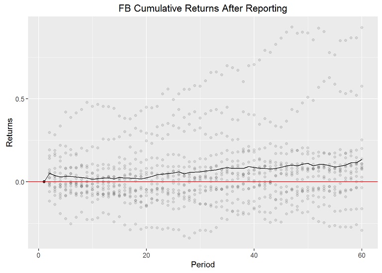
Boxplot of the first session after the release date:
period.data$period <- as.factor(period.data$period)
qplot(period, returns, data=period.data[period.data$period == 2,], geom=c("boxplot"),
   fill=period, main="First Session after Report",
   xlab="Period", ylab="Returns")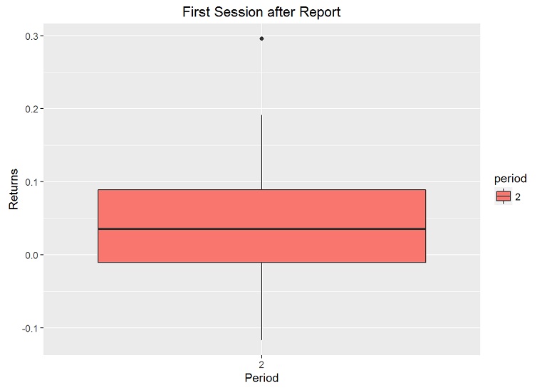
This shows the median price and where most of the prices (between the first and third quantile) lie.
Calculate the number of times the stock price increased the day after the report date:
nincreases <- sum(period.data[period.data$period == 2, "returns"] > 0)
nevents <- length(period.data[period.data$period == 2, "returns"])
ratio <- nincreases / nevents
Out of 16 previous reports, 10 times the next session increased, giving a ratio of 0.625.
The following boxplot shows how the price behaves over the following 23 sessions.
qplot(period, returns, data=period.data[period.data$period %in% as.character(2:24),], geom=c("boxplot"),
   fill=period, main="First 23 Periods After Earnings",
   xlab="Period", ylab="Returns")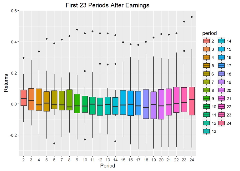
Conclusion
The plots tend to suggest that the stock price takes a bit of a dip between 7 and 14 days. This analysis isn’t to be used as an investment strategy. Much more analysis is needed before making investments, but it is interesting to see how the stock behaves after the report, and it would be interesting to see how other stocks behave after the report and compared to Facebook.
Justin Nafe July 31st, 2016
Posted In: Exploratory Analysis