Insights into data
Forecast Stock Prices Example with r and STL
Given a time series set of data with numerical values, we often immediately lean towards using forecasting to predict the future.
In this forecasting example, we will look at how to interpret the results from a forecast model and make modifications as needed. The forecast model we will use is stl().
Natural gas companies usually display a seasonal component, so we will evaluate the adjusted closing price of Northwest Natural Gas Co (NWN) from 1/1/2007 to 6/30/2016.
Load the data
library(quantmod)
library(xts)
library(tseries)
library(forecast)
library(timeSeries)


stock.symbols <- c("NWN")

stock.symbols.returned <- getSymbols(stock.symbols, from = "2007-01-01", to = "2016-06-30")

stock.data <- get(stock.symbols.returned[1])
Plot the time series
We got the daily prices from Yahoo. To take a quick look at the data, we can make a plot of the data.
chartSeries(stock.data, theme = "white", name = stock.symbols[1])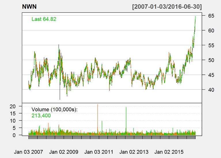
We will be evaluating the adjusted closing price, and we will convert the data to monthly data for better visuals.
stock.data.monthly <- to.monthly(stock.data)
adj <- Ad(stock.data.monthly)
The frequency parameter in ts() is the number of observations per unit of time. In this case, we use monthly data over a number of years, and want to detect seasons within a year, so we set the frequency to 12.
freq <- 12
adj.ts <- ts(adj, frequency = freq)
We want to create a training set and a testing set. The testing set will be used to test our forecast on data that the model did not see yet.
The timeSeries object is structured in such a way where the periods are the rows and the months are the columns. It would help us segment if we know how many periods there are and how many data points are in the partial period. Given that we know the frequency and the desired test size (3 months), we can calculate that information which will later be used to setup the test and training sets.
whole.periods <- floor(nrow(adj.ts) / freq)
partial.periods <- nrow(adj.ts) %% freq
With the timeseries we just created, the rows of the timeSeries object represent periods. We have to segment the timeSeries object with window and set the start and end parameters to row column vectors. Segmenting with window preserves the time series’ properties.
desired.test <- 3
training.end.row <- whole.periods + 1
training.end.col <- ifelse(partial.periods == 0, freq - desired.test, freq - partial.periods - desired.test)
if(partial.periods < desired.test){
  training.end.row <- whole.periods
  training.end.col <- freq - (desired.test - partial.periods)
}
training.ts <- window(adj.ts, c(1,1), c(training.end.row,training.end.col))
testing.ts <- window(adj.ts, c(training.end.row, training.end.col + 1))
Fit the Model
We will fit the model with STL. STL removes the seasonal component and leaves the randomness and trend. We will forecast with STL and arima with and without extra information, such as month.
Besides removing the seasonal component and then adding it back in after the predictions, STL also provides many parameters to help fine tune the training of our model. Some such parameters can allow us to have the seasonal component change over time, to handle the bias, to control the smoothness of the trend, to allow robustness to outliers, etc…
fit.stl <- stl(training.ts[,1], s.window = "period")Plot the decomposition.
plot(fit.stl, main="STL Decomposition")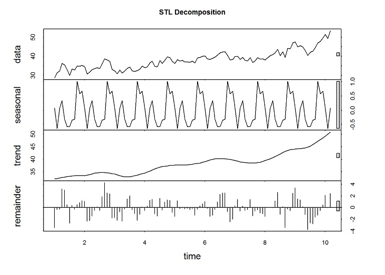
The spikes in the remainder are from the unusual spikes in the prices.
Forecast without month data
In this example, we will forecast the last 3 months to check the accuracy of the forecast.
forecasted.adj <- stlf(training.ts[,1], s.window = "period", method="arima", h=desired.test)
plot(forecasted.adj, main="Forecasts of NWN from STL and ARIMA (w/o month data)")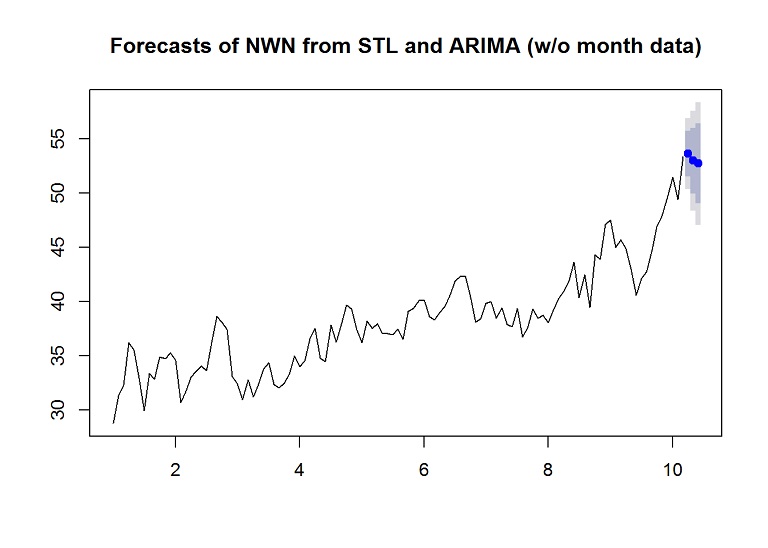
Evaluate the results
The residuals should be uncorrelated, else there is information left in the data that should be accounted for. Also the mean of the residuals should be zero, else the forecast is biased.
Check the accuracy
accuracy(forecasted.adj, testing.ts)## ME RMSE MAE MPE MAPE MASE
## Training set 0.2215072 1.650271 1.288773 0.4612967 3.405031 0.4448252
## Test set 3.9834881 7.183357 5.375876 6.0476637 8.749231 1.8555053
## ACF1 Theil's U
## Training set -0.11977014 NA
## Test set -0.03949848 1.164977Check the autocorrelation of the residuals
# Plot the residuals
res <- residuals(forecasted.adj)
plot(res, main="Residuals W/O Month Data and no Tuning")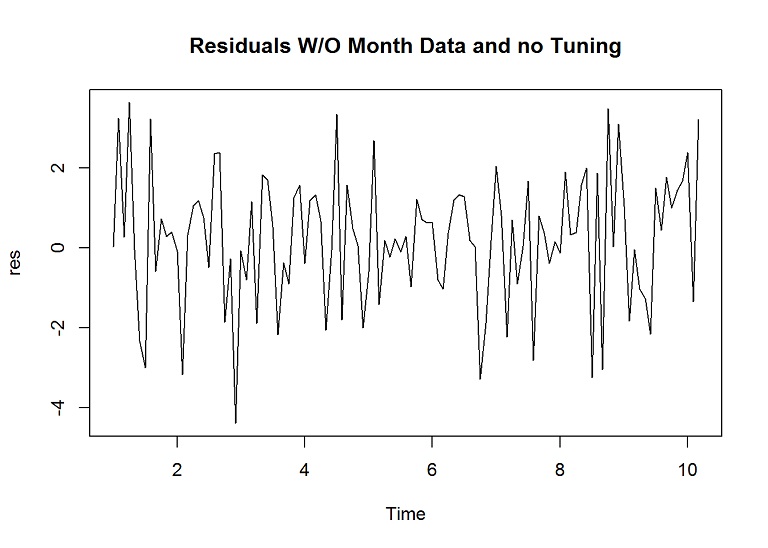
# Check the correlation of the residuals
Acf(res, main="Autocorrelation W/O Month Data and no Tuning")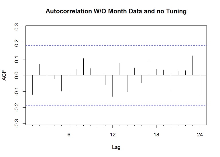
The lines don’t break above or below the dashed blue lines (a confidence level), so the lack of correlation suggests the forecast is good; however, a couple lines come close and we could improve this by setting the lambda parameter, which is used within the Box Cox transformation of the data before decomposition and then back.
Check the mean
mean(res)## [1] 0.2215072The mean is a bit more above zero than desired, so this means that the forecast is biased. One way to solve bias is to add the mean to all forecasts, but when using STL, and since we are transforming the data anyway, we will check the mean after tuning.
Tune the creation of the model
Let’s add the lambda parameter to the model building and forecasting to help reduce the correlation in the residuals and bring the residual mean closer to 0, and in effect improve the accuracy on the test set. I found that setting lambda to 1.9 for this dataset yielded the best results. I also found that setting robust to TRUE and biasadj to TRUE yielded the best results in reducing the mean of the residuals and minimizing the RMSE (balanced between the training set and the test set).
forecasted.adj <- stlf(training.ts[,1], s.window = "period", method="arima", h=desired.test, lambda = 1.9, robust = TRUE, biasadj = TRUE)
plot(forecasted.adj, main="Forecasts of NWN from tuned STL and ARIMA (w/o month data)")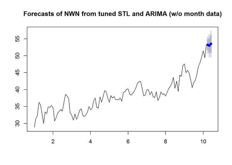
Check the accuracy
accuracy(forecasted.adj, testing.ts)## ME RMSE MAE MPE MAPE MASE
## Training set -0.01542828 1.685161 1.316494 -0.1832795 3.495005 0.4543933
## Test set 3.85330976 6.708538 4.973345 5.8986385 8.071776 1.7165702
## ACF1 Theil's U
## Training set 0.0149972 NA
## Test set -0.0421408 1.092232Check the autocorrelation of the residuals
# Plot the residuals
res <- residuals(forecasted.adj)

# Check the correlation of the residuals
Acf(res, main="Autocorrelation W/O Month Data and with Tuning")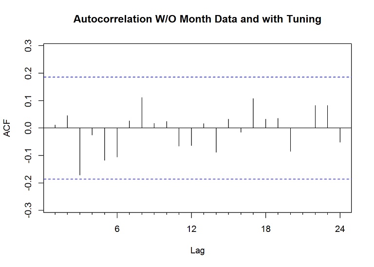
Check the mean
mean(res)## [1] 0.07549905The mean of the residuals is much closer to zero and the lines in the autocorrelation of the residuals are further away from the “confidence” lines.
Forecast with additional month data
dates <- index(adj)
months <- format(dates, "%b")

xreg.months <- model.matrix(~as.factor(months))[, 2:12]
colnames(xreg.months) <- gsub("as\\.factor\\(months\\)", "", colnames(xreg.months))
Setup the test and train datasets for the extra information
training.xtra <- xreg.months[1:nrow(training.ts),]
testing.xtra <- xreg.months[nrow(training.ts) + 1:nrow(testing.ts),]
Forecast with the additional data without some of the tuning parameters. The biasadj and robust parameters were not effective.
forecasted.adj <- stlf(training.ts[,1], s.window = "period", method="arima", h=nrow(testing.xtra), xreg = training.xtra, newxreg = testing.xtra, lambda = 1.5)
plot(forecasted.adj, main="Forecasts of NWN from STL and ARIMA (with month data)")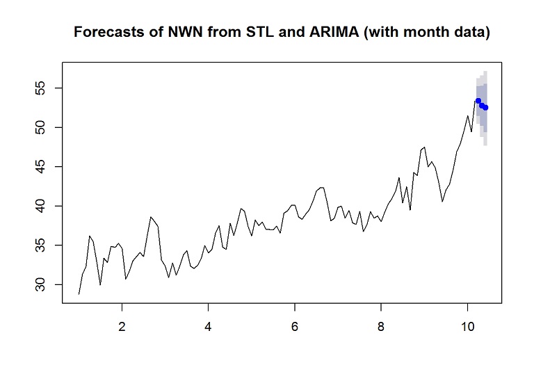
Evaluate the results
Check the accuracy
accuracy(forecasted.adj, testing.ts)## ME RMSE MAE MPE MAPE MASE
## Training set 0.2414978 1.640967 1.309111 0.5071425 3.460856 0.451845
## Test set 4.2038073 7.295160 5.425409 6.4398699 8.810071 1.872602
## ACF1 Theil's U
## Training set -0.007825514 NA
## Test set -0.040582743 1.187786If we look at the RMSE, the test set is worse with the extra month information.
Check the autocorrelation of the residuals
# Plot the residuals
res <- residuals(forecasted.adj)

# Check the correlation of the residuals
Acf(res, main="Autocorrelation with Month Data")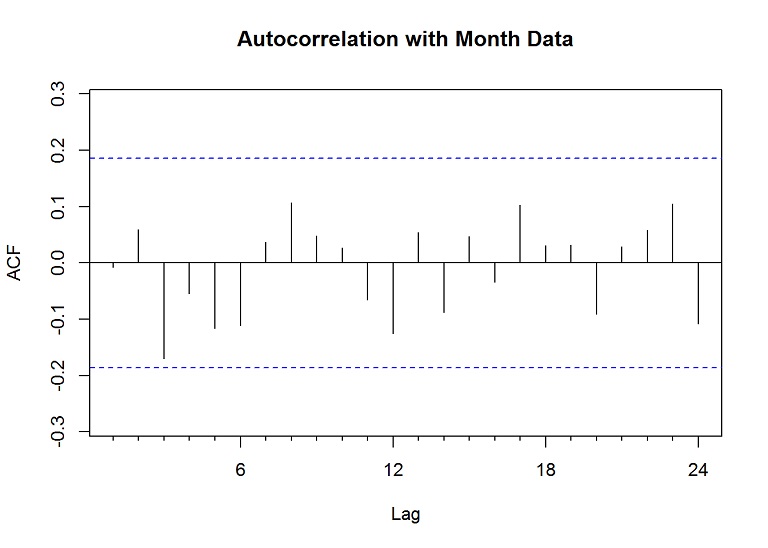
Check the mean
mean(res)## [1] 1.544952The mean of the residuals is much higher than zero, meaning the forecast is biased. We could attempt to tune the model more, try other stocks, or add more information, but I’ll leave that to you or another post later.
Justin Nafe July 8th, 2016
Posted In: Exploratory Analysis