Insights into data
Data Exploratory Analysis – Student Alcohol Consumption
Most of us experimented with drinking to some degree while in school. With the Student Alcohol Consumption data set from UCI Machine Learning Archive (Fabio Pagnotta 2016), we thought it would be interesting to see what features are important to determine if the student is a heavy drinker or not. With the Student Alcohol Consumption data set, we predict high or low alcohol consumption of students.
The original data comes from a survey conducted by a professor in Portugal. The primary reason for this data was to see the effects of drinking and grades. The data set consists of two files, one for students in a math class, and the other contains information about students in a Portuguese class.
Data Ingestion
The original data contains the following attributes for both student-mat.csv (Math course) and student-por.csv (Portuguese language course) datasets:
- school – student’s school (binary: ‘GP’ – Gabriel Pereira or ‘MS’ – Mousinho da Silveira)
- sex – student’s sex (binary: ‘F’ – female or ‘M’ – male)
- age – student’s age (numeric: from 15 to 22)
- address – student’s home address type (binary: ‘U’ – urban or ‘R’ – rural)
- famsize – family size (binary: ‘LE3’ – less or equal to 3 or ‘GT3’ – greater than 3)
- Pstatus – parent’s cohabitation status (binary: ‘T’ – living together or ‘A’ – apart)
- Medu – mother’s education (numeric: 0 – none, 1 – primary education (4th grade), 2 5th to 9th grade, 3 secondary education or 4 higher education)
- Fedu – father’s education (numeric: 0 – none, 1 – primary education (4th grade), 2 5th to 9th grade, 3 secondary education or 4 higher education)
- Mjob – mother’s job (nominal: ‘teacher’, ‘health’ care related, civil ‘services’ (e.g. administrative or police), ‘at_home’ or ‘other’)
- Fjob – father’s job (nominal: ‘teacher’, ‘health’ care related, civil ‘services’ (e.g. administrative or police), ‘at_home’ or ‘other’)
- reason – reason to choose this school (nominal: close to ‘home’, school ‘reputation’, ‘course’ preference or ‘other’)
- guardian – student’s guardian (nominal: ‘mother’, ‘father’ or ‘other’)
- traveltime – home to school travel time (numeric: 1 – <15 min., 2 – 15 to 30 min., 3 – 30 min. to 1 hour, or 4 – >1 hour)
- studytime – weekly study time (numeric: 1 – <2 hours, 2 – 2 to 5 hours, 3 – 5 to 10 hours, or 4 – >10 hours)
- failures – number of past class failures (numeric: n if 1<=n<3, else 4)
- schoolsup – extra educational support (binary: yes or no)
- famsup – family educational support (binary: yes or no)
- paid – extra paid classes within the course subject (Math or Portuguese) (binary: yes or no)
- activities – extra-curricular activities (binary: yes or no)
- nursery – attended nursery school (binary: yes or no)
- higher – wants to take higher education (binary: yes or no)
- internet – Internet access at home (binary: yes or no)
- romantic – with a romantic relationship (binary: yes or no)
- famrel – quality of family relationships (numeric: from 1 – very bad to 5 – excellent)
- freetime – free time after school (numeric: from 1 – very low to 5 – very high)
- goout – going out with friends (numeric: from 1 – very low to 5 – very high)
- Dalc – workday alcohol consumption (numeric: from 1 – very low to 5 – very high)
- Walc – weekend alcohol consumption (numeric: from 1 – very low to 5 – very high)
- health – current health status (numeric: from 1 – very bad to 5 – very good)
- absences – number of school absences (numeric: from 0 to 93)
The following grades are related with the course subject, Math or Portuguese:
- G1 – first period grade (numeric: from 0 to 20)
- G2 – second period grade (numeric: from 0 to 20)
- G3 – final grade (numeric: from 0 to 20, output target)
Data Import
Before exploration, we combine the rows of the two data sets and mark each instance with the class in which the survey was taken. We could perform this merge differently later by performing a full join and then dealing with the NA values, by performing the analysis on the individual sets, or by inner joining the two sets and just working with that data. For this analysis, we combine the rows of the data sets.
By stacking one data set on top of the other, we assume that each instance is not an instance for the student, but an instance of when the student completed the survey.
por <- read.csv("..\\..\\Data\\Common\\UCI_Alcohol_Consumption\\student-por.csv", sep = ";")
mat <- read.csv("..\\..\\Data\\Common\\UCI_Alcohol_Consumption\\student-mat.csv", sep = ";")

por$math_instance <- 0
mat$math_instance <- 1

data <- rbind(por, mat)
The target is the weekday drinking level 1 to 5 and the weekend drinking level 1 to 5. Since we attempt to predict the students’ level of alcohol consumption, high or low, we mutate the targets to join the weekday and weekend drinking, and then set the results to high or low, 1 or 0 respectively.
This modification coincides with the original report where the authors modified the target with the formula acl = (Dalc * 5 + Walc * 2) / 7 and then assumed values of 3 or more were heavy drinkers.
data$alc <- ifelse(((data$Dalc * 5 + data$Walc * 2) / 7) < 3, 0, 1)
data$Walc <- NULL
data$Dalc <- NULL
Data Configuration
We prefer to use some sort of configuration so that we can input any dataset and perform most of the same analysis. Yaml is a good tool for setting up configurations, but in this case, we will set the configurations manually.
# detect data types
isNumerical = sapply(data, is.numeric)
isCategorical = sapply(data,function(x)length(unique(na.omit(x)))<=nrow(data)/500||length(unique(na.omit(x)))<=5)
isNumerical = isNumerical & !isCategorical
colNames = colnames(data)

config <- list()
config$CategoricalColumns <- c("alc")
config$Target <- "alc"

if(!is.null(config$CategoricalColumns)){
  config$CategoricalColumns = make.names(config$CategoricalColumns, unique=TRUE)
  for(v in config$CategoricalColumns){
    isCategorical[v] = TRUE;
    isNumerical[v] = FALSE;
  }
}

if(!is.null(config$NumericalColumns)){
  config$NumericalColumns = make.names(config$NumericalColumns, unique = TRUE)
  for(v in config$NumericalColumns){
    isNumerical[v] = TRUE;
    isCategorical[v] = FALSE;
    }
}

config$CategoricalColumns = colNames[isCategorical[colNames] == TRUE]
config$NumericalColumns = colNames[isNumerical[colNames] == TRUE]

for(v in config$CategoricalColumns)
{
   data[,v] = as.factor(data[,v])
}


# detect task type
if(is.null(config$Target)){
  taskType = 'data_exploration'
} else if(isCategorical[config$Target]==FALSE){
  taskType='regression'
} else {
  taskType='classification'
}
Data Summary
Quick Data Description
- The target is – alc
- The task type is – classification.
- The numerical variables are – age, absences, G1, G2, G3
- The categorical variables are – school, sex, address, famsize, Pstatus, Medu, Fedu, Mjob, Fjob, reason, guardian, traveltime, studytime, failures, schoolsup, famsup, paid, activities, nursery, higher, internet, romantic, famrel, freetime, goout, health, math_instance, alc
Basic Statistics
The data that we will explore has 1044 rows and 33 columns.
The types of columns are listed as follows:
# get the data type of each column
 Column_Type = sapply(data, class)
 Column_Type = lapply(Column_Type, function(x) paste(x, collapse=' '))
 column_info = cbind(Column_Name= names(Column_Type), Column_Type)
 rownames(column_info) <- NULL
 column_info[1:nrow(column_info),]
## Column_Name Column_Type
## [1,] "school" "factor"
## [2,] "sex" "factor"
## [3,] "age" "integer"
## [4,] "address" "factor"
## [5,] "famsize" "factor"
## [6,] "Pstatus" "factor"
## [7,] "Medu" "factor"
## [8,] "Fedu" "factor"
## [9,] "Mjob" "factor"
## [10,] "Fjob" "factor"
## [11,] "reason" "factor"
## [12,] "guardian" "factor"
## [13,] "traveltime" "factor"
## [14,] "studytime" "factor"
## [15,] "failures" "factor"
## [16,] "schoolsup" "factor"
## [17,] "famsup" "factor"
## [18,] "paid" "factor"
## [19,] "activities" "factor"
## [20,] "nursery" "factor"
## [21,] "higher" "factor"
## [22,] "internet" "factor"
## [23,] "romantic" "factor"
## [24,] "famrel" "factor"
## [25,] "freetime" "factor"
## [26,] "goout" "factor"
## [27,] "health" "factor"
## [28,] "absences" "integer"
## [29,] "G1" "integer"
## [30,] "G2" "integer"
## [31,] "G3" "integer"
## [32,] "math_instance" "factor"
## [33,] "alc" "factor"One way to get an idea about the structure of the data is to calculate basic statistics, such as the min, max, mean, and median, and missing value counts. This information can give you a hint of the skewness and of possible outliers. The following shows basic statistics of each feature:
summary(data)## school sex age address famsize Pstatus Medu
## GP:772 F:591 Min. :15.00 R:285 GT3:738 A:121 0: 9
## MS:272 M:453 1st Qu.:16.00 U:759 LE3:306 T:923 1:202
## Median :17.00 2:289
## Mean :16.73 3:238
## 3rd Qu.:18.00 4:306
## Max. :22.00
## Fedu Mjob Fjob reason guardian
## 0: 9 at_home :194 at_home : 62 course :430 father:243
## 1:256 health : 82 health : 41 home :258 mother:728
## 2:324 other :399 other :584 other :108 other : 73
## 3:231 services:239 services:292 reputation:248
## 4:224 teacher :130 teacher : 65
##
## traveltime studytime failures schoolsup famsup paid activities
## 1:623 1:317 0:861 no :925 no :404 no :824 no :528
## 2:320 2:503 1:120 yes:119 yes:640 yes:220 yes:516
## 3: 77 3:162 2: 33
## 4: 24 4: 62 3: 30
##
##
## nursery higher internet romantic famrel freetime goout health
## no :209 no : 89 no :217 no :673 1: 30 1: 64 1: 71 1:137
## yes:835 yes:955 yes:827 yes:371 2: 47 2:171 2:248 2:123
## 3:169 3:408 3:335 3:215
## 4:512 4:293 4:227 4:174
## 5:286 5:108 5:163 5:395
##
## absences G1 G2 G3
## Min. : 0.000 Min. : 0.00 Min. : 0.00 Min. : 0.00
## 1st Qu.: 0.000 1st Qu.: 9.00 1st Qu.: 9.00 1st Qu.:10.00
## Median : 2.000 Median :11.00 Median :11.00 Median :11.00
## Mean : 4.435 Mean :11.21 Mean :11.25 Mean :11.34
## 3rd Qu.: 6.000 3rd Qu.:13.00 3rd Qu.:13.00 3rd Qu.:14.00
## Max. :75.000 Max. :19.00 Max. :19.00 Max. :20.00
## math_instance alc
## 0:649 0:926
## 1:395 1:118
##
##
##
## Addressing skewness, the mean of absences is 4.4348659 and the median is 2, indicating that the data is right-skewed and given the spread between the min and max, the skewness is significant. We will take a closer look at the distribution of this feature.
The following results show the skewness for the numeric features:
library(e1071)
apply(data[,isNumerical], 2, skewness)
## age absences G1 G2 G3
## 0.43278208 3.73060247 0.07769868 -0.49592905 -0.98313324As we suspected, the feature ‘absences’ contains the most skew.
Distribution
We look a bit closer at the distribution of absences and test for normality. Depending on the model you choose, removing skewness could help improve the predictive ability of the model.
plotNormality <- function(dataVector, colName){
  par(mfrow=c(2,2))
  normtest <- shapiro.test(dataVector)

  p.value <- round(normtest$p.value,4)
  if (p.value < 0.05) {
    h0 <- 'rejected.'
    color <- 'red'
  } else {
    h0 <- 'accepted.'
    color <- 'blue'
  }
  hist(dataVector, xlab = colName, main = paste('Histogram of', colName))

  d <- density(dataVector)
  plot(d, main = paste('Density Plot of ', colName))
  qqnorm(dataVector, main = paste('QQ Plot of', colName))
  qqline(dataVector)
  boxplot(dataVector, main = paste('Boxplot of', colName))
  mtext(paste('Normality test of ', colName, ' ', h0, ' (p-value=', p.value, ')', sep=''), side = 3, line = -1, outer = TRUE, col=color)
}
plotNormality(data[['absences']], 'absences')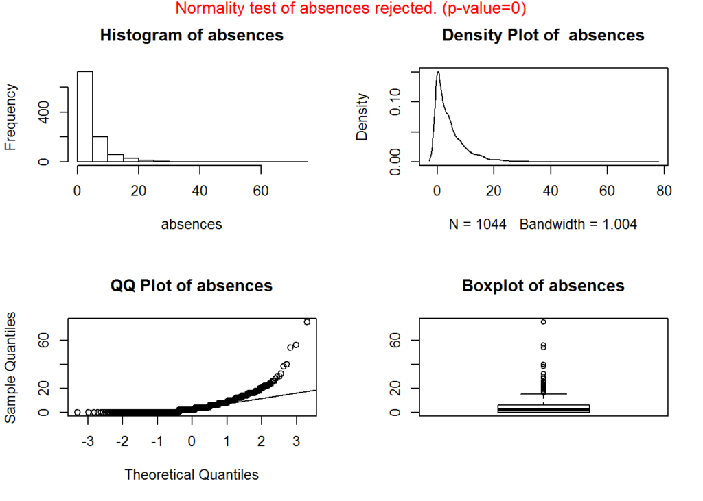
We remove skewness by applying a log, square root, or/and inverse transformation. Since the distribution is log normal, applying the log transformation would be the most applicable.
absenceLogged <- log(data[['absences']] + 1)
plotNormality(absenceLogged, 'absences logged')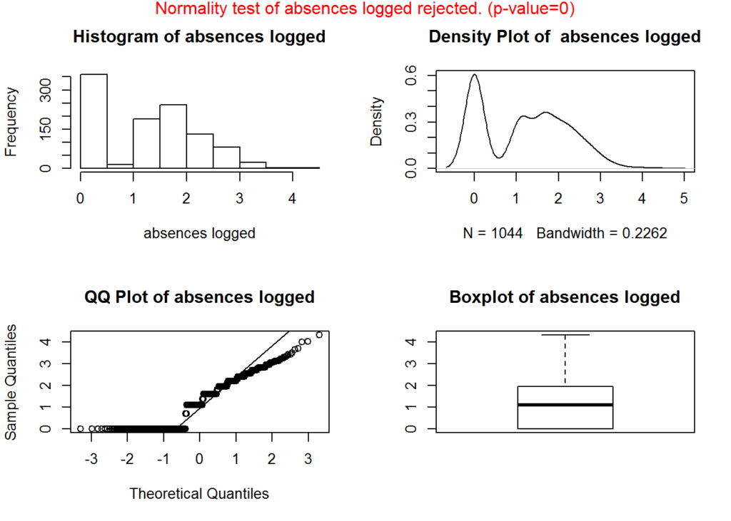
To test this, we will also apply the Box and Cox method to determine the parameter that indicates which method is best. We only do this for illustration. The original values for the feature ‘absences’ will be used in the remaining sections.
library(caret)
absenceTransormed <- BoxCoxTrans(data[['absences']] + 1)
absenceTransormed
## Box-Cox Transformation
##
## 1044 data points used to estimate Lambda
##
## Input data summary:
## Min. 1st Qu. Median Mean 3rd Qu. Max.
## 1.000 1.000 3.000 5.435 7.000 76.000
##
## Largest/Smallest: 76
## Sample Skewness: 3.73
##
## Estimated Lambda: -0.1
## With fudge factor, Lambda = 0 will be used for transformationsWhen lambda = 0, the log transform is used.
Target
The following plot shows the prominence of the target:
    par(mfrow=c(1, 2))
    barplot(table(data[[config$Target]]), main = paste('Bar Plot of', config$Target), col=c("lightblue", "lightgreen"))
pie(table(data[[config$Target]]), main=paste('Pie Chart of', config$Target), col=c("lightblue", "lightgreen")) 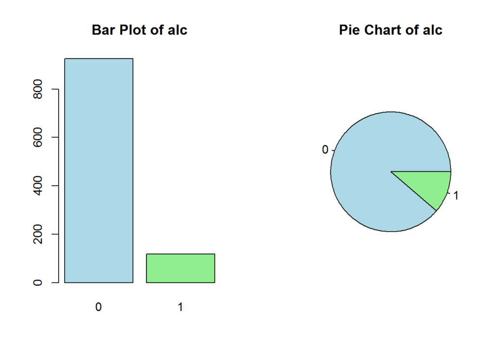
This shows that the target is imbalanced, so we may benefit from oversampling or under-sampling when building our model. We would oversample since we have limited data.
Feature Interactions
Rank associated features
To get an idea of how features interact with each-other, we can determine the rank associated with the features to a target, in this case, the actual target or level of drinking.
This helps you to understand the top dependent variables (grouped by numerical and categorical). If one is very high, you may want to take a closer look at the data and see if there is leakage into the target variable. For categorical values, we use Cramer’s V. For numeric values, we use Eta-squared value
    library(parallel)
    library(doSNOW)
     par(mfrow=c(1,2))
  no_cores <- max(detectCores() - 1, 1)
  cluster <- makeCluster(no_cores)
  registerDoSNOW(cluster)
  if(isCategorical['alc'] == TRUE){
    aov_v <- foreach(i=1:length(config$NumericalColumns),.export=c('config','data'),.packages=c('DescTools'),.combine='c') %dopar%
    {
      get('config')
      get('data')
      if (max(data[[config$NumericalColumns[i]]]) != min(data[[config$NumericalColumns[i]]]))
      {
        col1 <- data[[config$NumericalColumns[i]]]
        index1 <- is.na(col1)
        col1[index1] <- 0
        fit <- aov(col1 ~ data[['alc']])
        EtaSq(fit)[1]

      } else{
        0
      }
    }
    names(aov_v) = config$NumericalColumns
    aov_v = subset(aov_v, names(aov_v)!='alc')
    aov_v = sort(aov_v, decreasing = TRUE)
    barplot(head(aov_v, 7), xlab = '', beside=TRUE, main = paste('Top', length(head(aov_v, 7)), 'Numerical Features'), las=2, col=c("lightblue", "lightgreen"))

    cramer_v <- foreach(i=1:length(config$CategoricalColumns), .export=c('config','data'), .combine='c') %dopar%
    {
      get('config')
      get('data')
      data[,config$CategoricalColumns[i]] <- factor(data[,config$CategoricalColumns[i]])
      if (nlevels(data[,config$CategoricalColumns[i]]) >= 2)
      {
        tbl = table(data[,c('alc', config$CategoricalColumns[i])])
        chi2 = chisq.test(tbl, correct=F)
        sqrt(chi2$statistic / sum(tbl))
      } else{
        0
      }

    }
    names(cramer_v) = config$CategoricalColumns
    cramer_v = subset(cramer_v, names(cramer_v)!='alc')
    cramer_v = sort(cramer_v, decreasing = TRUE)
    barplot(head(cramer_v, 7), xlab = '', beside=TRUE, main = paste('Top', length(head(cramer_v, 7)), 'Categorical Features'), las=2, col=c("lightblue", "lightgreen"))


}![]()
stopCluster(cluster)The results make sense. According to the World Health Organization (Global Status Report on Alcohol and Health 2014 2014), gender, family, and social factors affect alcohol consumption.
Correlations (numerical)
For numeric data, correlations are important to help determine if we should join information of highly correlated features.
In this case, we see that the grades are highly correlated, meaning the higher the grades in one session, the higher the grades in another session. You can see the level of correlation by the degree of the ellipse. The more narrow the ellipse, the stronger the correlation.
library(corrgram)
library(corrplot)
par(mfrow=c(1,1))
c = cor(data[,config$NumericalColumns], method = 'pearson')
corrplot(c, method='ellipse', order = 'AOE', insig = 'p-value',  sig.level=-1, type = 'full')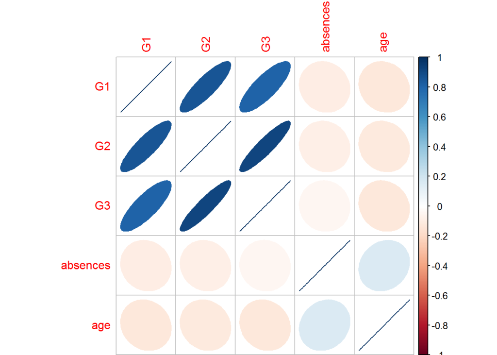
You may want to explore combining the grades into one feature since G3 is likely derived from G1 and G2. Generally, many models prefer using features that are independent of each other and have low correlations. For example, if there were a high correlation, say 0.9, between two numeric features, then the information provided to the model would be redundant, and depending on the model make the model more complex than it needs to be.
Associations (categorical)
To compare categorical variables, correlations shouldn’t be used unless the underlying values are ordinal (i.e., going out with friends [numeric: from 1 – very low to 5 – very high]). In our data set, many of the categorical features are numeric, but for this illustration, we will continue with treating them as categorical.
We assume that a father’s education level is similar to a mother’s education level, so let us visualize the association:
library(vcd)
par(mfrow=c(1,1))
mosaicplot(table(data[['Medu']], data[['Fedu']]),  shade=TRUE, xlab='Medu', ylab='Fedu', main=paste('Medu','VS', 'Fedu'))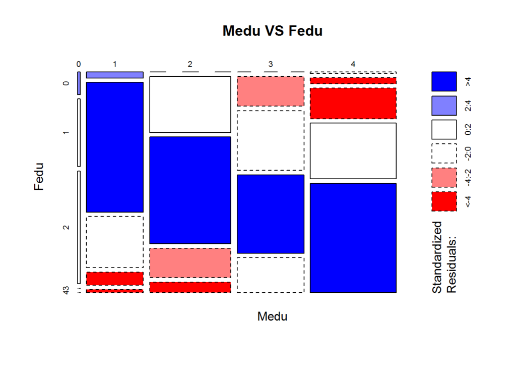
The above plot shows that the education levels between mother and father do coincide fairly often and might want to explore more or consider the possibility of joining these features in preprocessing the data before model building. Essentially, the blue rectangles show that the observed counts and expected counts (derived from a loglinear model) coincide well, and since the size of the rectangles are large, the confidence covers a majority of the observations.
Violin / box plots with target
X axis is the level of categorical target. This helps you to understand whether the distribution of the numeric variable is significantly different at different levels of the categorical target.
We test hypothesis 0 (h0) that the numeric variable has the same mean values across the different levels of the categorical variable. If the mean has significant differences (h0 is accepted), then the feature will likely be a dominant predictor.
The box plot portion of the graph also helps us identify outliers.
library(ggplot2)

plotViolins <- function(df, num, cat){
  fit <- aov(df[[num]] ~ df[[cat]])
    test_results <- drop1(fit,~.,test='F')
    p_value <- round(test_results[[6]][2],4)
    if (p_value < 0.05){
      h0 <- 'Rejected'
      color <- 'red'
    } else{
      h0 <- 'Accepted'
      color <- 'blue'
    }
    ggplot(df, aes(x = factor(cat), y = df[,num], fill = factor(df[,cat]))) +
    geom_violin(aes(y = df[,num], x = df[,cat], fill = factor(df[,cat]))) +
    geom_boxplot(aes(y = df[,num], x = df[,cat]), width=.1) +
    theme(legend.position = "none") +
    theme(plot.subtitle=element_text(size=8, hjust=0.5, face="italic", color=color)) +
    labs(x=cat, y=num, title=paste("Violin Plot of ", cat, " and ", num, sep = ""), subtitle=paste('Violin Plot h0 ', h0, ' (p-value=', p_value, ')',sep=''))
}
multiplot <- function(..., plotlist=NULL, file, cols=1, layout=NULL) {
  library(grid)

  # Make a list from the ... arguments and plotlist
  plots <- c(list(...), plotlist)

  numPlots = length(plots)

  # If layout is NULL, then use 'cols' to determine layout
  if (is.null(layout)) {
    # Make the panel
    # ncol: Number of columns of plots
    # nrow: Number of rows needed, calculated from # of cols
    layout <- matrix(seq(1, cols * ceiling(numPlots/cols)),
                    ncol = cols, nrow = ceiling(numPlots/cols))
  }

 if (numPlots==1) {
    print(plots[[1]])

  } else {
    # Set up the page
    grid.newpage()
    pushViewport(viewport(layout = grid.layout(nrow(layout), ncol(layout))))

    # Make each plot, in the correct location
    for (i in 1:numPlots) {
      # Get the i,j matrix positions of the regions that contain this subplot
      matchidx <- as.data.frame(which(layout == i, arr.ind = TRUE))

      print(plots[[i]], vp = viewport(layout.pos.row = matchidx$row,
                                      layout.pos.col = matchidx$col))
    }
  }
}

p1 <- plotViolins(data, 'absences', 'alc')
p2 <- plotViolins(data, 'age', 'alc')
multiplot(p1, p2, cols = 2)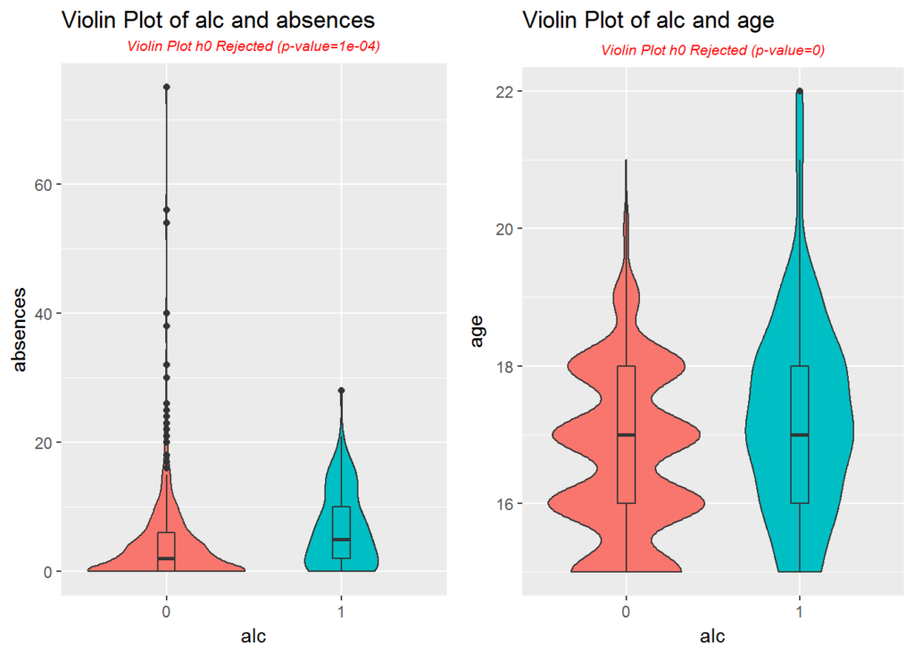
The violin plot of absences shows more of a log normal distribution, and a large number of outliers lie well outside of the top whisker. We may want to normalize absences in preparation for model building.
p3 <- plotViolins(data, 'G1', 'alc')
p4 <- plotViolins(data, 'G2', 'alc')
p5 <- plotViolins(data, 'G3', 'alc')
multiplot(p3, p4, p5, cols = 3)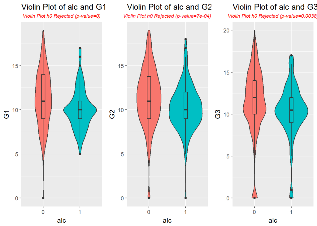
Conclusion
Next Steps in Preparing the Data for a Model
From this analysis, what might we preprocess before creating the model?
Remove the skewness from the numeric data. Modify the number features by:
- Joining information from existing features (PCA is a common example, or some knowledge about how features are correlated)
- Depending on the model, remove features that are not important to the model
Depending on the algorithms used in the model building, the following features may produces better results as numeric and normalized. Many of them are ordinal and were discretized from continuous values.
- Fedu
- Medu
- traveltime
- studytime
- failures
- famrel
- freetime
- goout
- health
Fedu and Medu correlate more that some others, so we might want to combine the information. One way would be to create a new feature, FeduMedu, where the values is Medu * 10 + Fedu and keep FeduMedu categorical.
References
Fabio Pagnotta, Hossain Mohammad Amran. 2016. “Using Data Mining to Predict Secondary School Student Alcohol Consumption.” Department of Computer Science,University of Camerino. https://archive.ics.uci.edu/ml/datasets/STUDENT%20ALCOHOL%20CONSUMPTION.
Global Status Report on Alcohol and Health 2014. 2014. World Health Organization WHO. http://www.who.int/substance_abuse/publications/global_alcohol_report/en/.
Justin Nafe December 21st, 2016
Posted In: Exploratory Analysis
Tags: r