Insights into data
How to use linear regression to predict housing prices
So far, I’ve taken a few of machine learning classes, all from Coursera, and all of them started with predicting house prices with linear regression to get us started with machine learning.
For those of you that would like to get an in-depth look at Machine Learning, I would recommend the Machine Learning class taught by Andrew Ng. It is a very resource intensive class, resources being the time spent on the assignments and learning.
I assume all the classes start with regression because linear regression is a powerful tool, can be used on many datasets, and is easy to understand.
Linear regression is commonly used to predict house prices. There are other models that we could use to predict house prices, but really, the model you choose depends on the dataset that you are using and which model is the best fit on the training data and the withheld test data.
What makes this post different than every other post about linear regression and house prices? Not much, but the post walks you through most of the process that I commonly take when evaluating data and creating predictive models.
I prefer to at least perform the following, usually repeating many times as I gather more data or end up changing the data in any way.
- Gather the data.
- Explore the data using visualizations and statistics, such as correlations.
- Clean up the data, such as decide what to do with missing values, misspellings, features that have no variance, etc…
- Wrangle the data. Create new features out of the data at hand
- Build the predictive model, often using a best guess approach based on the type of data and output. For example, image data would likely include a nueral network, finite output would likely involve classification, and numerical output would likely involve some form of regression.
- Tune the model and use cross validation.
- Evaluate the model. I often use the RMSE or ROC, again depending on the data.
I prefer to use caret because it provides us with many model options and tuning parameters and provides us with a simple means to evaluate models.
The dataset we will be using http://wiki.csc.calpoly.edu/datasets/attachment/wiki/Houses/RealEstate.csv?format=raw from the wiki.csc.calpoly.edu. Or it can be downloaded from here. The data is quite old but for illustration purposes, it should be fine.
library(ggplot2)
library(tabplot)
library(caret)

data <- read.csv("http://wiki.csc.calpoly.edu/datasets/attachment/wiki/Houses/RealEstate.csv?format=raw", stringsAsFactors = FALSE)
Data exploration
Once the data is downloaded, take an initial look at the data, structure of the data, missing values, etc…
We start by exploring the data and cleaning up if necessary.
head(data)## MLS Location Price Bedrooms Bathrooms Size Price.SQ.Ft
## 1 132842 Arroyo Grande 795000 3 3 2371 335.30
## 2 134364 Paso Robles 399000 4 3 2818 141.59
## 3 135141 Paso Robles 545000 4 3 3032 179.75
## 4 135712 Morro Bay 909000 4 4 3540 256.78
## 5 136282 Santa Maria-Orcutt 109900 3 1 1249 87.99
## 6 136431 Oceano 324900 3 3 1800 180.50
## Status
## 1 Short Sale
## 2 Short Sale
## 3 Short Sale
## 4 Short Sale
## 5 Short Sale
## 6 Short Saledim(data)## [1] 781 8summary(data)## MLS Location Price Bedrooms
## Min. :132842 Length:781 Min. : 26500 Min. : 0.000
## 1st Qu.:149922 Class :character 1st Qu.: 199000 1st Qu.: 3.000
## Median :152581 Mode :character Median : 295000 Median : 3.000
## Mean :151225 Mean : 383329 Mean : 3.142
## 3rd Qu.:154167 3rd Qu.: 429000 3rd Qu.: 4.000
## Max. :154580 Max. :5499000 Max. :10.000
## Bathrooms Size Price.SQ.Ft Status
## Min. : 1.000 Min. : 120 Min. : 19.33 Length:781
## 1st Qu.: 2.000 1st Qu.:1218 1st Qu.: 142.14 Class :character
## Median : 2.000 Median :1550 Median : 188.36 Mode :character
## Mean : 2.356 Mean :1755 Mean : 213.13
## 3rd Qu.: 3.000 3rd Qu.:2032 3rd Qu.: 245.42
## Max. :11.000 Max. :6800 Max. :1144.64From the summary of the data, we can tell that there are no missing values, so we don’t need to worry about what to do with them.
str(data)## 'data.frame': 781 obs. of 8 variables:
## $ MLS : int 132842 134364 135141 135712 136282 136431 137036 137090 137159 137570 ...
## $ Location : chr "Arroyo Grande" "Paso Robles" "Paso Robles" "Morro Bay" ...
## $ Price : num 795000 399000 545000 909000 109900 ...
## $ Bedrooms : int 3 4 4 4 3 3 4 3 4 3 ...
## $ Bathrooms : int 3 3 3 4 1 3 2 2 3 2 ...
## $ Size : int 2371 2818 3032 3540 1249 1800 1603 1450 3360 1323 ...
## $ Price.SQ.Ft: num 335 142 180 257 88 ...
## $ Status : chr "Short Sale" "Short Sale" "Short Sale" "Short Sale" ...unique(data$Location)## [1] "Arroyo Grande" "Paso Robles" "Morro Bay"
## [4] "Santa Maria-Orcutt" "Oceano" "Atascadero"
## [7] "Los Alamos" "San Miguel" "San Luis Obispo"
## [10] "Cayucos" "Pismo Beach" "Nipomo"
## [13] "Guadalupe" "Los Osos" "Templeton"
## [16] "Grover Beach" "Cambria" "Solvang"
## [19] "Bradley" "Avila Beach" "Santa Ynez"
## [22] "King City" "Creston" "Lompoc"
## [25] "Coalinga" "Buellton" "Lockwood"
## [28] "Greenfield" "Soledad" "Santa Margarita"
## [31] "Bakersfield" "New Cuyama" " Lompoc"
## [34] " Nipomo" " Arroyo Grande" "San Simeon"
## [37] " Morro Bay" " Pismo Beach" " Cambria"
## [40] " Paso Robles" " Out Of Area" " Los Osos"
## [43] " Santa Maria-Orcutt" " Grover Beach" " Templeton"
## [46] " Atascadero" " Oceano" " Cayucos"
## [49] " Creston" "Out Of Area" " San Luis Obispo"
## [52] " Solvang" " Bradley" " San Miguel"It looks like there are some spaces in the beginning of the some of the Locations, creating separate locations for the same location. For example “Morro Bay” and " Morro Bay" should be “Morro Bay”
data$Location <- gsub("^ ", "", data$Location)

unique(data$Location)
## [1] "Arroyo Grande" "Paso Robles" "Morro Bay"
## [4] "Santa Maria-Orcutt" "Oceano" "Atascadero"
## [7] "Los Alamos" "San Miguel" "San Luis Obispo"
## [10] "Cayucos" "Pismo Beach" "Nipomo"
## [13] "Guadalupe" "Los Osos" "Templeton"
## [16] "Grover Beach" "Cambria" "Solvang"
## [19] "Bradley" "Avila Beach" "Santa Ynez"
## [22] "King City" "Creston" "Lompoc"
## [25] "Coalinga" "Buellton" "Lockwood"
## [28] "Greenfield" "Soledad" "Santa Margarita"
## [31] "Bakersfield" "New Cuyama" "San Simeon"
## [34] "Out Of Area"Let’s try to detect visual correlations for the numeric data. We will exlude the MLS number since that is an id and will not contribute to our prediction. Also, since we are trying to predict price, the price per sq ft shouldn’t be known. In other words, when trying to predict y, in this case Price, the features need to be independent of Price. Price per sq ft is dependent on price and should not be a feature, so price per sq ft will excluded.
# Exclude price per sq ft
data$Price.SQ.Ft <- NULL

# Remove MLS
data$MLS <- NULL
Plot the numeric data and output the correlations to check for bivariate correlations.
nums <- sapply(data, is.numeric)
plot(data[,nums])cor(data[,nums])## Price Bedrooms Bathrooms Size
## Price 1.0000000 0.2531624 0.5201100 0.6647236
## Bedrooms 0.2531624 1.0000000 0.5883705 0.5970701
## Bathrooms 0.5201100 0.5883705 1.0000000 0.7615426
## Size 0.6647236 0.5970701 0.7615426 1.0000000Size and Bathrooms are highly correlated (a cutoff that I commonly use is +-0.7), so it might be worthwhile to try and combine the two and see the effect on our prediction model. We will try using principle component analysis for that latter.
Check if any of the features have a near zero variance.
nearZeroVar(data[, -2], saveMetrics = TRUE)## freqRatio percentUnique zeroVar nzv
## Location 2.780000 4.3533931 FALSE FALSE
## Bedrooms 2.435028 1.1523688 FALSE FALSE
## Bathrooms 1.964602 1.0243278 FALSE FALSE
## Size 1.500000 67.4775928 FALSE FALSE
## Status 3.185185 0.3841229 FALSE FALSEtableplot(data)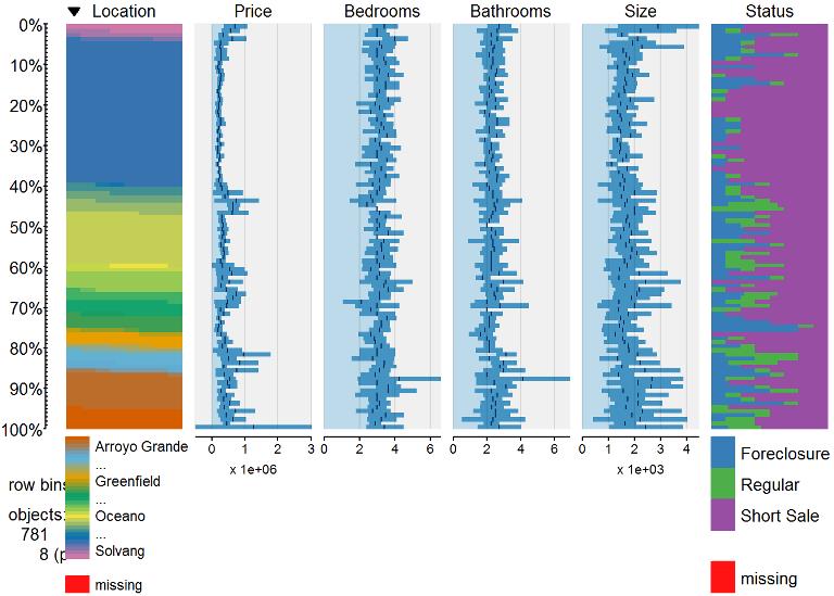
If any did have near zero variance, then we would consider removing that feature.
If using linear regression, Location as a feature, and principle component analysis (PCA); we want to make sure that each feature is seen enough times in training so that there are no near zero variance for each location, otherwise we get errors when the test set contains a categorical feature not seen before or the model is not optimal. We will find cases where location is used only a few times and then remove those rows for this example; otherwise you might want to combine those locations with ones that are very similar to the other features and price. Or feel free to comment your ideas and I’ll revisit this post.
freq <- as.data.frame(table(data$Location))
loc <- freq[freq$Freq > 3,]
loc
## Var1 Freq
## 1 Arroyo Grande 40
## 2 Atascadero 68
## 5 Bradley 4
## 6 Buellton 12
## 7 Cambria 21
## 9 Coalinga 7
## 12 Grover Beach 22
## 13 Guadalupe 4
## 16 Lompoc 27
## 18 Los Osos 27
## 19 Morro Bay 17
## 21 Nipomo 37
## 22 Oceano 11
## 23 Out Of Area 4
## 24 Paso Robles 100
## 25 Pismo Beach 20
## 26 San Luis Obispo 17
## 27 San Miguel 15
## 30 Santa Maria-Orcutt 278
## 31 Santa Ynez 5
## 33 Solvang 10
## 34 Templeton 12data <- data[data$Location %in% loc$Var1, ]
# Check how many rows we have now
nrow(data)## [1] 758It looks like we removed about 6 rows.
Size appears to be most correlated with price, so let’s plot a scatter plot to see the distribution
plot(data$Size, data$Price, main="Price and Sq Ft",
     xlab="Sq Ft ", ylab="Price", pch=19)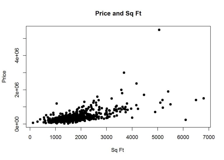
With just size, let’s do a simple prediction model with just the size.
Partition the data
First we partition the data into test and training sets.
set.seed(3456)
trainIndex <- createDataPartition(data$Price, p = .8,
                                  list = FALSE,
                                  times = 1)

train <- data[ trainIndex,]
test  <- data[-trainIndex,]
Cross validate
Then we can setup some cross validation. I have not run into a case where it is not a good idea to cross validate.
# Create 10 folds of cross validation.
fitControl <- trainControl(
  method = "cv")
Create models and predict
Train the simple model and make predictions with size and price.
simplemodel <- train(Price~Size, train, method = "lm", trControl = fitControl)

pred <- predict(simplemodel, test)
To evaluate the model on the actual test set, get the RMSE on the test set.
RMSE(pred, test$Price)## [1] 196063.4Plot the test data with the predicted values
plot(test$Size, test$Price, main="Price and Sq Ft",
     xlab="Sq Ft ", ylab="Price", pch=19)
abline(simplemodel$finalModel$coefficients, col="red")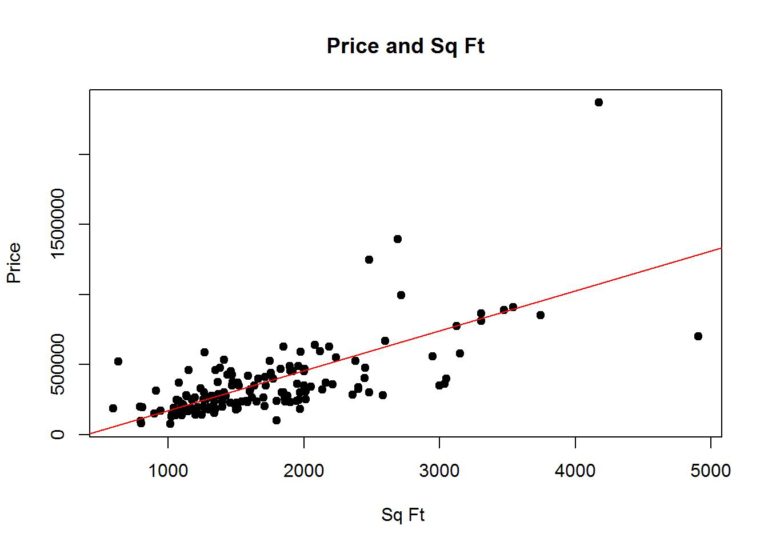
Let’s add some features to see if we can reduce the RMSE. First let’s take a look at the data and how it is distributed. Boxplots can be used to find outliers, but we will not be removing the outliers in this example.
boxplot(data$Size)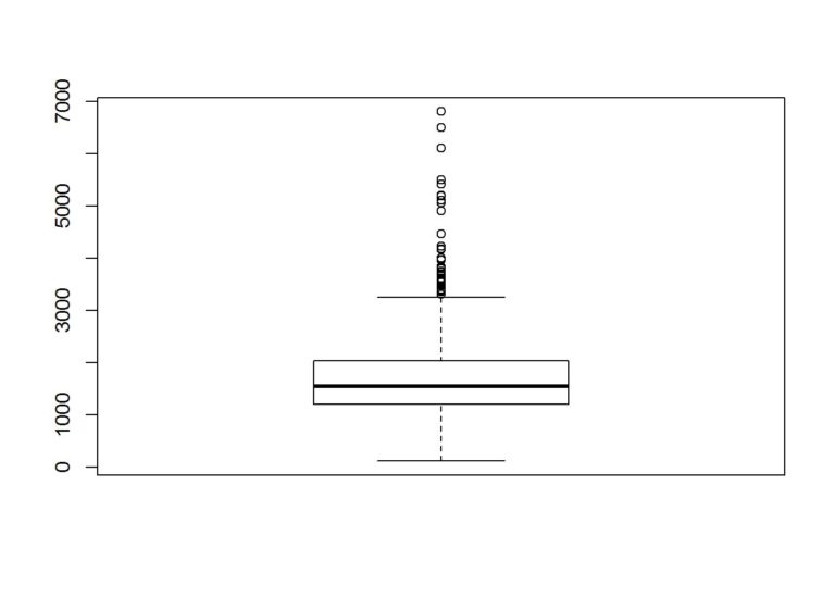
boxplot(Price~Status, data = data)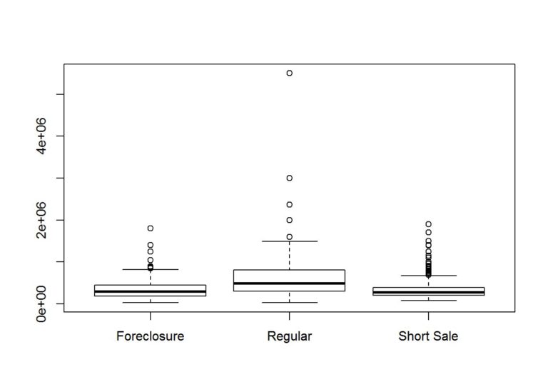
boxplot(Price~Bedrooms, data = data)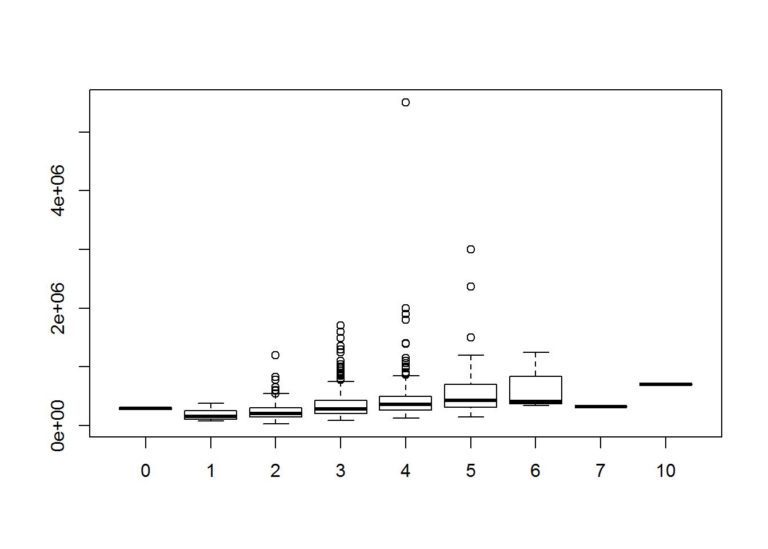
boxplot(Price~Bathrooms, data = data)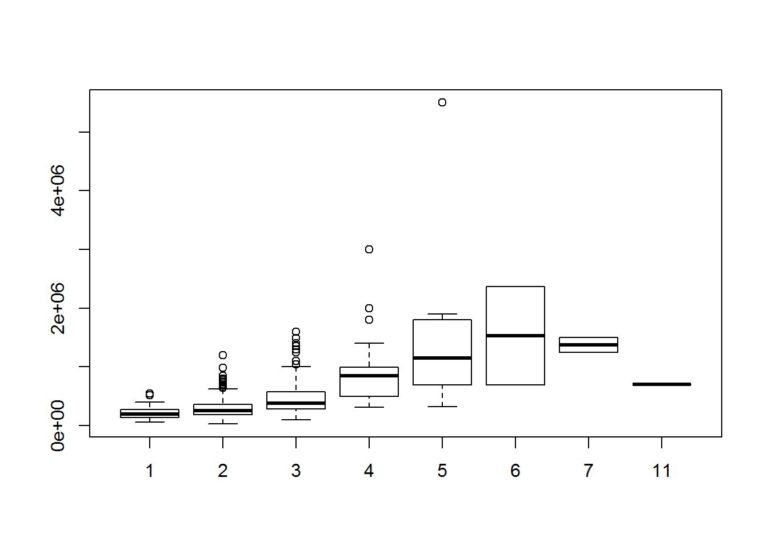
Train with the additional features.
set.seed(3456)
allfeaturesmodel <- train(Price~., train, method = "lm", trControl = fitControl)
Compare the two models we created. We use RMSE when comparing models that are attempting to predict the same thing, in this case the price of the house. Also, comparing regression models by the RMSE is helpful because they are in the same units as the predicted value.
allfeaturesmodel## Linear Regression
##
## 607 samples
## 5 predictor
##
## No pre-processing
## Resampling: Cross-Validated (10 fold)
## Summary of sample sizes: 546, 546, 546, 547, 545, 547, ...
## Resampling results
##
## RMSE Rsquared RMSE SD Rsquared SD
## 213326.7 0.6668864 127122.3 0.1280567
##
## simplemodel## Linear Regression
##
## 607 samples
## 5 predictor
##
## No pre-processing
## Resampling: Cross-Validated (10 fold)
## Summary of sample sizes: 545, 546, 546, 546, 547, 547, ...
## Resampling results
##
## RMSE Rsquared RMSE SD Rsquared SD
## 250944.2 0.5082873 129186.2 0.1227094
##
## Run the test data using the new model
allFeaturesPred <- predict(allfeaturesmodel, test)To evaluate the model on the actual test set, get the RMSE on the test set.
RMSE(allFeaturesPred, test$Price)## [1] 157477.3Looks like using the model with more features minimized the RMSE for the training set and test set, so we are on the right track.
Just for curiosity, what are the important or most predictive features? Since we used non numeric features, caret creates dummy variables out of the non-numeric features.
varImp(allfeaturesmodel$finalModel)## Overall
## LocationAtascadero 4.4423588
## LocationBradley 1.0383573
## LocationBuellton 1.8043828
## LocationCambria 1.3487699
## LocationCoalinga 3.1381742
## `LocationGrover Beach` 1.8246608
## LocationGuadalupe 1.5888109
## LocationLompoc 4.1415339
## `LocationLos Osos` 2.8896773
## `LocationMorro Bay` 0.6038438
## LocationNipomo 3.2257274
## LocationOceano 0.1111560
## `LocationOut Of Area` 2.6122182
## `LocationPaso Robles` 5.2700601
## `LocationPismo Beach` 0.6629921
## `LocationSan Luis Obispo` 0.6733428
## `LocationSan Miguel` 3.5476783
## `LocationSanta Maria-Orcutt` 6.6992176
## `LocationSanta Ynez` 0.9327655
## LocationSolvang 1.8863275
## LocationTempleton 2.3401892
## Bedrooms 2.0284754
## Bathrooms 1.3988614
## Size 13.0463927
## StatusRegular 4.6695966
## `StatusShort Sale` 0.4908264Earlier, I mentioned that a couple of the features had a high correlation. To combine features that have a high correlation, I prefer to use principle component analysis; however, if I have to explain the most predictive features, PCA makes it more difficult.
set.seed(3456)
pcamodel <- train(Price~., train, method = "lm", trControl = fitControl, preProcess = "pca" )
pcaPred <- predict(pcamodel, test)
Now let’s compare all models and test results.
simplemodel## Linear Regression
##
## 607 samples
## 5 predictor
##
## No pre-processing
## Resampling: Cross-Validated (10 fold)
## Summary of sample sizes: 545, 546, 546, 546, 547, 547, ...
## Resampling results
##
## RMSE Rsquared RMSE SD Rsquared SD
## 250944.2 0.5082873 129186.2 0.1227094
##
## allfeaturesmodel## Linear Regression
##
## 607 samples
## 5 predictor
##
## No pre-processing
## Resampling: Cross-Validated (10 fold)
## Summary of sample sizes: 546, 546, 546, 547, 545, 547, ...
## Resampling results
##
## RMSE Rsquared RMSE SD Rsquared SD
## 213326.7 0.6668864 127122.3 0.1280567
##
## pcamodel## Linear Regression
##
## 607 samples
## 5 predictor
##
## Pre-processing: principal component signal extraction (26), centered
## (26), scaled (26)
## Resampling: Cross-Validated (10 fold)
## Summary of sample sizes: 546, 546, 546, 547, 545, 547, ...
## Resampling results
##
## RMSE Rsquared RMSE SD Rsquared SD
## 225201.1 0.6100417 133813.2 0.137512
##
## RMSE(pred, test$Price)## [1] 196063.4RMSE(allFeaturesPred, test$Price)## [1] 157477.3RMSE(pcaPred, test$Price)## [1] 196635.5It looks like combining highly correlated features did not help in this case, but of course we could always tune the model more or try different models.
To elaborate on an earlier comment about using PCA makes it difficult to explain the features that are important; you can print out the coefficients and see why.
coefficients(pcamodel$finalModel)## (Intercept) PC1 PC2 PC3 PC4 PC5
## 386146.191 -143970.851 59160.269 -7158.715 69742.997 39347.169
## PC6 PC7 PC8 PC9 PC10 PC11
## -28504.671 24639.000 27146.600 -14101.467 11932.950 11686.614
## PC12 PC13 PC14 PC15 PC16 PC17
## 7920.247 -12628.547 16115.118 22314.222 4256.158 10559.176
## PC18 PC19 PC20 PC21 PC22
## -11700.790 -31003.622 13418.905 32756.097 11006.390As you can see, a lot of creating a good model involves trial and error, but so long as you evaluate your model and results, you can come to an adequate model. In this case, a tree model, such as random forest, would fit the data better than the models created in this post, but the post is about linear regression.
Hopefully this helps someone learning the basics. Feel free to comment about how to improve this analysis using linear regression
Justin Nafe May 30th, 2016
Posted In: Exploratory Analysis, Machine Learning
Tags: linear regression, r