Insights into data
Impute Data with Related Features
Much of the data that we use for exploratory analysis is missing data. One way to handle the missing data is to impute it. We will use related data to impute crime locations.
What if we could determine the type of crime, forecast when a type of crime would happen again in a certain location or at a time of day, or what crimes are most predictable, or what features are most predictive of crimes? Maybe crime fighting could be improved, but this isn’t the first time people tried to address these issues. Simply googling forecast crime will render many interesting results.
Dallas Open Data now supplies a fairly thorough record of the crimes committed in Dallas county, it is their RMS system. You can download the data, filter the data with an API, and explore the data, which is what we will start to do in this post, and eventually fine tune our data exploration and prediction/forecasting of crimes.
The crime records give us dates and times of the call or report, the complainant information such as name and address, the crime that was committed, location, reporting officers, and much more. For this post about exploratory analysis, we focus on location and time of crime to prepare for crime type prediction.
Load Dallas Crime Data
We download the full dataset so that we can explore the data with different features or methods latter. The full dataset is large and may take a while. I end up saving the data to a file to use again latter.
library(cluster)
library(fpc)
library(scales)
library(lubridate)
library(caret)


rms.file <- "rms.csv"
if(!file.exists(rms.file)){
  download.file("http://www.dallasopendata.com/api/views/tbnj-w5hb/rows.csv?accessType=DOWNLOAD",
                destfile=rms.file)
}
crime.data <- read.csv("rms.csv", na.strings = "" )
I chose to import strings as factors so that when we run summary(crime.data), we can see the number of na values.
Goal of Imputing Location Information
Ultimately, we want to answer many interesting questions, but a large part of exploring data is coming up with new predictive features, handling missing data, etc… For this analysis, we will be handling missing TAAG data (locations defined by the police department) by imputing the data via clustering. This may not be the best way to handle the missing data, but it is one way and I’d be interested in hearing other ways to handle the TAAG missing data.
Subset Location and Time Features
We can start by removing the columns that are specifically associated or dependent on the predicted variable. The features that we are going to use should be independent of the dependent predicted variable. We will look at variables such as time, date, location. In a follow-up post, we will be predicting the type of offense, so UCROffense is included.
crime.data <- crime.data[,c("PointX", "PointY", "TAAG",
                            "Date1", "Year1", "Month1", "Day1", "Time1", "UCROffense")]
Data Cleanup and Wrangling
Before splitting the dataset up into test and train, we will do any cleanup or data wrangling on the set, such as add a column hour, day of month. We also impute the missing TAAG data.
crime.data$Date1 <- strptime(crime.data$Date1, format = "%m/%d/%Y %I:%M:%S %p")

crime.data$Hour <- strptime(crime.data$Time1, format = "%H:%M")

crime.data$Hour <- hour(crime.data$Hour)
crime.data$Hour <- as.numeric(crime.data$Hour)

crime.data$DayOfMonth <- day(crime.data$Date1)
crime.data$DayOfMonth <- as.numeric(crime.data$DayOfMonth)
After changing the data, let’s print a summary to see what information is missing or to see data that doesn’t make sense.
summary(crime.data)## PointX PointY TAAG
## Min. :2411659 Min. :6886689 Ross Bennett : 5572
## 1st Qu.:2477174 1st Qu.:6954767 Forest Audelia : 5316
## Median :2493382 Median :6976138 Central CFHawn : 5068
## Mean :2494683 Mean :6978314 CampWisdom Chaucer: 5009
## 3rd Qu.:2508872 3rd Qu.:7002055 Five Points : 4306
## Max. :2595095 Max. :7083051 (Other) :82071
## NA's :6455 NA's :6455 NA's :85467
## Date1 Year1 Month1
## Min. :1989-01-27 00:00:00 Min. :1989 May : 17099
## 1st Qu.:2014-12-06 00:00:00 1st Qu.:2014 December: 17088
## Median :2015-06-15 00:00:00 Median :2015 October : 16885
## Mean :2015-06-07 02:30:33 Mean :2015 January : 16630
## 3rd Qu.:2015-12-09 00:00:00 3rd Qu.:2015 July : 16443
## Max. :2016-06-03 00:00:00 Max. :2016 (Other) :108663
## NA's :1 NA's :1 NA's : 1
## Day1 Time1 UCROffense
## Fri :29516 00:00 : 6675 THEFT/BMV :30111
## Sat :28394 22:00 : 5636 VANDALISM & CRIM MISCHIEF:20711
## Mon :27284 18:00 : 5373 ACCIDENT MV :15533
## Wed :27016 17:00 : 4965 BURGLARY-RESIDENCE :15461
## Thu :26964 20:00 : 4865 FOUND :15144
## (Other):53634 (Other):165294 OTHER THEFTS :13692
## NA's : 1 NA's : 1 (Other) :82157
## Hour DayOfMonth
## Min. : 0.00 Min. : 1.00
## 1st Qu.: 8.00 1st Qu.: 8.00
## Median :14.00 Median :16.00
## Mean :12.83 Mean :15.69
## 3rd Qu.:19.00 3rd Qu.:23.00
## Max. :23.00 Max. :31.00
## NA's :1 NA's :1There are quite a few data points that are missing, and some that don’t make any sense, such as
TAAG
Targeted Area Action Grids (TAAG) account for approximately half of the locations. TAAG was derived to help focus on crime reduction in hot spots around Dallas. They achieve this goal by setting up cameras, placing cars in locations that have a high probability of getting broken into, etc…
Many locations and crimes committed therein don’t belong to a TAAG, so we will try to create new areas by clustering non TAAG locations and see if the new tags help with predicting the type of crime (the prediction part will be posted latter).
Unfortunately, the dataset doesn’t use lat long values, but instead use a proprietary X and Y coordinate system. This makes it more difficult to map out the locations of the TAAGs or locations of the new clusters without knowing what the x and y coordinates translate to on the lat long coordinate system (this will be handled in another post).
There are 48 unique TAAGs and they are mapped out differently. In other words, without knowing how these TAAGs are determined, a quick and dirty way to create pseudo TAAGs for the missing values would be to cluster the missing values. We have 48 TAAG values, and a little under half of the crimes have a TAAG value. So we could try to best fit the missing values using k-means with a k value based on results within sum of squares.
#initialize the new collumn
crime.data$PseudoTAAG <- crime.data$TAAG

# let's remove the rows that have missing values for PointX and PointY
crime.data <- crime.data[!is.na(crime.data$PointX) & !is.na(crime.data$PointY),]

wss <- (nrow(crime.data[is.na(crime.data$PseudoTAAG),])-1)*sum(apply(crime.data[is.na(crime.data$PseudoTAAG),c("PointX", "PointY")],2,var))
for (i in 2:60) wss[i] <- sum(kmeans(crime.data[is.na(crime.data$PseudoTAAG),c("PointX", "PointY")], centers=i)$withinss)
plot(1:60, wss, type="b", xlab="Number of Clusters",
     ylab="Within groups sum of squares")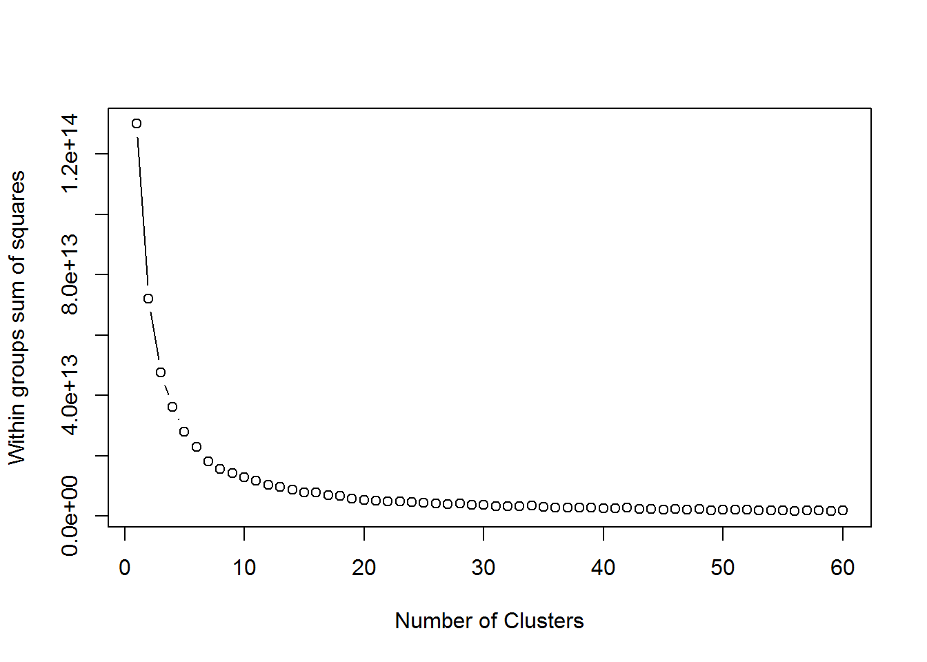
Using the elbow method of evaluating the number of center points in the k-means, about 10 clusters is optimal for the missing TAAG values. Remember that they are likely not derived in the same way as the existing TAAG values.
k <- 10

set.seed(1234)
taagClusters <- kmeans(crime.data[is.na(crime.data$PseudoTAAG),c("PointX", "PointY")], centers=k)
crime.data$PseudoTAAG <- as.character(crime.data$PseudoTAAG)
subsetForPlot <- crime.data[is.na(crime.data$PseudoTAAG),]
subsetForPlot[, "PseudoTAAG"] <- as.character(taagClusters$cluster)
crime.data[is.na(crime.data$PseudoTAAG), "PseudoTAAG"] <- as.character(taagClusters$cluster)
crime.data$PseudoTAAG <- as.factor(crime.data$PseudoTAAG)

plot(subsetForPlot[,c("PointX", "PointY")],
     col = alpha(taagClusters$cluster, 0.1),
     pch = 20, cex = 3)
points(taagClusters$centers, pch = 4, cex = 4, lwd = 4 )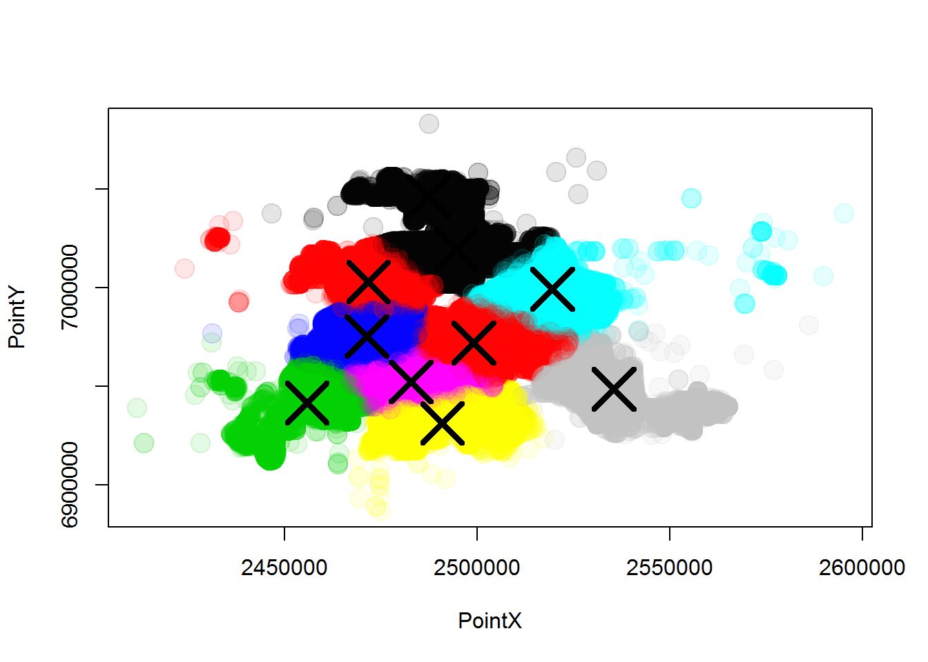
Now we have “TAAG” values (in the PseudoTAAG column) for every crime that has an xy coordinate. There are many ways to impute data for missing values, but this is an example of one way to impute where we use related data. In a latter post, we will evaluate the effectiveness of imputing using this method on this dataset.
Justin Nafe June 5th, 2016
Posted In: Exploratory Analysis
Tags: clustering, r